Pipeline Data Flow in Disco Jobs

The dataflow and computation in a Disco job is structured as a pipeline, where a pipeline is a linear sequence of stages, and the outputs of each stage are grouped into the inputs of the subsequent stage.

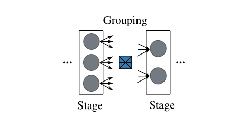
The high-level idea of a pipeline is shown below:

It can also be represented succinctly as follows:

pipeline  ::=  stage+
stage     ::=  {grouping, task}

A stage consists of a set of tasks that perform the same computation, but on different inputs. For example, a map stage can consist of a set of Map tasks, each of which takes in a single input, whereas a reduce stage typically consists of a single Reduce task that can process all the inputs to the reduce stage.

A grouping operation specifies how the inputs to a stage are divided into inputs for the tasks that belong to that stage. The grouping of a set of inputs is performed using the label attached to each input.

The outputs generated by the tasks in a stage become the inputs for the tasks in the subsequent stage of the pipeline. Whenever a task generates an output file, it attaches an integer label to that file. These labeled outputs become the labeled inputs for the grouping operation performed by the subsequent stage.

In other words, a pipeline is a sequence of stages, and each stage performs a grouping of its labeled inputs into one or more groups. Each such group of inputs is processed by a single task, whose definition is part of the definition of the stage.

There are five different grouping operations that the user can choose for a stage: split, group_node, group_label, group_node_label, and group_all. Each of these operations take in a set of inputs, and group them using the labels attached to each input and the cluster node on which the input resides. (Note: inputs not residing on a known cluster node, e.g. those that are specified using http:// URLs that point outside the cluster, are currently treated as residing on a single fictitious cluster node.)

The simplest ones are split, group_all and group_label, since they do not take into account the cluster node on which the inputs reside, so lets explain them first.

Split

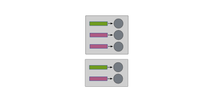
The split operation puts each input into its own group, regardless of the label of the input, or the cluster node on which it resides. The grey boxes below indicate the cluster nodes on which the inputs reside, while labels are indicated by the colors of the inputs.

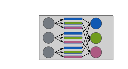
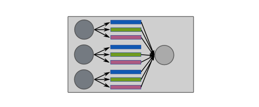
Group_all

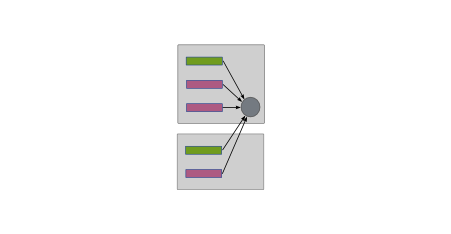
The group_all operation puts all inputs into a single group, again regardless of their labels or hosting cluster nodes, illustrated below.

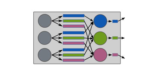
Group_label

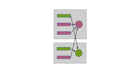
On the other hand, the group_label operation takes into account the labels, and puts all inputs with the same label into the same group. As before, this is done without regard to the cluster nodes hosting the inputs, below.

Map-Reduce

To illustrate the pipeline model, we can now use it to express a simple Map-Reduce job, show below, with job inputs and outputs shown in black.

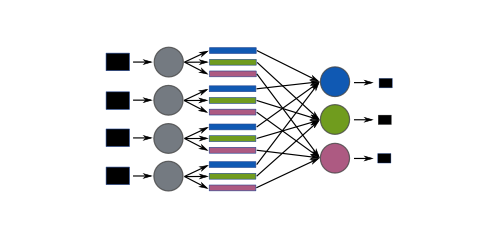
When expressed as a pipeline, this becomes simply:

map-reduce = {split, <map>}, {group_label, <reduce>}

The first stage, <map>, of this pipeline puts each input to the pipeline into its own group, and executes a <map> task with that group as input. Each <map> task produces a set of labeled outputs. These labeled outputs become the labeled inputs of the <reduce> stage. This <reduce> stage puts all inputs with the same label into a single group, and executes a <reduce> task that takes in each such group as input. Hence, the number of such <reduce> tasks is determined by the number of distinct labels generated by the <map> tasks in the <map> stage. The labeled outputs generated by the <reduce> tasks in the <reduce> stage become the outputs of the map-reduce pipeline. This shows how the normal Partitioned Reduce DataFlow in earlier versions of Disco can be implemented.

Let’s now clarify one issue that might be raised at this point: the inputs to the pipeline are not the outputs of a previous stage in the pipeline, so what labels are attached to them? The answer is that the labels for the job inputs are derived from The Job Pack submitted to Disco by the user, and hence are user-specified. (However, see the discussion of backward-compatibility issues in The Job Pack.)

One issue that may be clear from the diagram is that the group_label operation, also known as shuffle in map-reduce terminology, can involve a lot of network traffic. It would be nice to optimize the network transfers involved. Indeed, that is precisely what the remaining grouping operations will let us do.

Group_label_node

The group_label_node operation is essentially the group_label operation, but performed on every cluster node.

We can use this operation to condense intermediate data belonging to the same label and residing on the same node, before the data is transmitted across the network.

We can use this in the map-reduce pipeline by adding an additional stage with this grouping operation:

map-condense-reduce = {split, <map>}, {group_node_label, <condense>}, {group_label, <reduce>}

Group_node

The last grouping operation, group__node, similarly is essentially the group_all operation, but performed on every cluster node.

This provides an alternative to group_node_label to users when trying to condense intermediate data on a node-local basis. The choice between the two will be determined by the fact that a group_node_label stage will typically have more tasks each of which will process less data (and hence probably have lower memory requirements) than a corresponding group_node stage.

It should be clear now that the five grouping operations provide the user a range of complementary options in constructing a flexible data processing pipeline.